
Getting Started
Get in Touch
Where we’re located:
We live, work, and play in beautiful Tallahassee, Florida.
Billing & Payment Mailing Address:
2910 Kerry Forest Pkwy, D4-282
Tallahassee, FL 32309 USA
We are SOC 2 Compliant

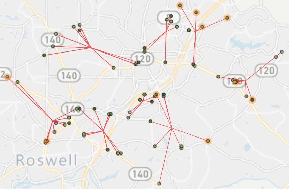
One of the powerful features of EasyTerritory is partitioning. Partitioning divides point locations on a map into sets (clusters) of equal workload. A workload is computed by totaling the onsite times and estimated drive-times between each stop in the partition. An ideal partitioning of a set of points is easy to imagine; they are isolated, small and equal in workload. Take for example a set of customer work-orders for servicing point-of-sale equipment. In this example, ideally the service technicians are not crossing each other in transit; they are driving the fewest number of miles and they are spending the same number of hours working and driving. Though easy to imagine, it’s hard to determine without a software like EasyTerritory.
In real-world scenarios, ideal partitioning is rarely achieved. There are almost always compromises. The primary compromise revolves around the tension between small, isolated partitions — we will call these clusters — and equally-distributed workloads. Nearly all scenarios allow for good clustering or equal-distribution, but not both. Some scenarios allow for a good compromise where both are more than acceptable. Other scenarios must be analyzed to determine which compromise is most acceptable. In EasyTerritory, this analysis requires the user to adjust the sliding scale between “cluster” and “distribute” when partitioning.
![]()
So what happens when you move the slider? That’s a good question and many of our customers leave it balanced in the middle as they are not sure what to set it to. But here’s how it works. If the slider is moved to the left it will bias the partitioning engine towards clustering, resulting in smaller, isolated partitions. Your service techs are not passing each other and their total workload is minimized. Great! But the downside is an increased variance in the cluster’s total workload — total onsite time plus total drive time. One service tech might have an 8-hour day and another a 6-hour day.
![]()
If the slider is moved to the right, the partitioning engine is biased towards distribution, resulting in partitions of equal workload. All of your service techs have roughly 7 hours of driving and on-site time. Super! But the downside here is the partitions are larger (more drive-time) and they are more likely to overlap. You look at the results and you wonder why one service tech is assigned to a stop deep inside another technician’s route. But that is the mathematical compromise that cannot be escaped in most scenarios.
![]()
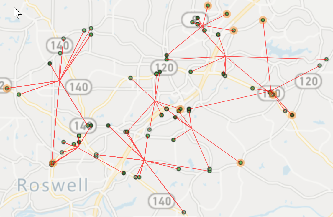
So how do planners determine the level of compromise? The challenge is in determining distribution — clustering is simple. For clustering, you simply look at the map in EasyTerritory. If they are less isolated, larger and have more overlap, then you know you are compromising on total drive-times and encroachment and clustering is not optimal. If the partitions are smaller and more isolated, then you know you are maximizing drive-time efficiency and reducing encroachment.
For distribution, the planner is shown CoV in real time as the partitioning engine is running. CoV is the coefficient-of-variation, or sometimes called relative-standard-deviation. The lower the CoV the better. Because it is relative-standard-deviation, (standard-deviation divided by the mean) it always provides a useful value that is more industry-dependent than scenario-dependent. In other words, if a planner finds the partitioning results for scenario A to have a good workload distribution and the CoV is 0.02, then if it is 0.02 in scenario B, the distribution is also likely to be acceptable. The planner will need to try a few scenarios to see how CoV corresponds with what is acceptable in their business practice.
To determine in absolute terms (in hours) each partitioned workload, you have two options. If you bring up the partitions properties in the markup panel in EasyTerritory, you will see a total-time estimate. You can compare these between partitions to determine the quality of distribution. The only way to get a solid comparison is to fine-route each partition using the EasyTerritory routing capabilities. This will give you the most accurate analysis of how well your partitions are distributed.
Finally, the density of stops makes a difference. If your accounts are located miles apart in rural areas (lower density) then you will typically want to bias more towards distribution. Due to the large variance in drive-times, small isolated clusters are almost certainly going to vary greatly in hours of workload. If your scenarios are in metro-areas with many accounts close-by (higher density), then you will likely want to bias more towards clustering. Drive-time is less of a factor and overlap between partitions is more likely.
If you are new to partitioning, a good first step is simply experiment with your data until you get comfortable with the settings and the results. If you find the results are generally good but need a few tweaks, EasyTerritory provides a manual means to address this. Please see our videos on partitioning for more information.